Optical Science Laboratory
Surface acoustic waves (SAWs) provide a dynamic one- or two-dimensional
lateral modulation of the band structure of quantum wells (QWs) [1, 2].
In this study, we investigate the dynamic optical properties of excitons
in GaAs/AlAs moving dots (dynamic quantum dots, DQDs) formed by the interference
of orthogonally propagating SAW beams. The SAWs induce a strain as well
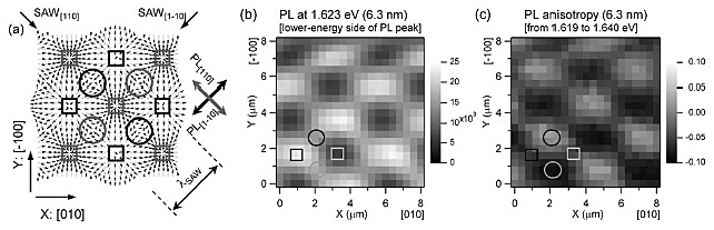
as a piezoelectric modulation of the materials properties. Due to the D4d symmetry of the underlying GaAs crystal, the interference of the two orthogonal
SAW beams leads to the formation of two interpenetrating square arrays
of DQDs [3], as shown in Fig. 1(a), where the in-plane components of the
particle displacement field are shown schematically. One of the arrays
(black and gray circles) consists of potential dynamic dots (p-DDs) created
by the modulation of the piezoelectric potential. The second array (black
and gray squares) is composed of strain dynamic dots (s-DDs), where the
band gap becomes minimum or maximum due to the modulation of the hydrostatic
strain.
Spatially resolved photoluminescence (PL) measurement at 4 K was carried out by using a synchronized excitation method [1]. Figure 1(b) shows the PL mapping for a 6.3-nm QW recorded at a photon energy of 1.623 eV, which is located in the lower-energy side of the PL peak (centered at 1.630 eV in the absence of a SAW). In the PL polarization studies, we define the degree of polarization anisotropy ρ as the relative difference ρ = (PL[1-10] - PL[110]) / ( PL[1-10] + PL[110]) between the PL intensity emitted along the [1-10] (PL[1-10]) and [110] (PL[110]) propagation directions of the individual SAW beam. Figures 1 (b) and
(c) clearly demonstrate the formation of the two DQD arrays. The strong
and weak PL positions in Fig. 1(b) correspond to the tensile (black squares
in Fig. 1(a)) and compressive (gray squares in Fig. 1(a)) s-DD positions,
respectively. In contrast, the positive (negative) ρ areas in Fig. 1 (c) are located at the saddle point of the tensile s-DDs
along the [1-10] ([110]) direction, denoted by a black (gray) circle in
Figs. 1 (b) and (c). The positions with strong PL anisotropy correspond
to the array of the p-DDs.
[1] T. Sogawa et al., Phys. Rev. B 80 (2009) 075304.
[2] T. Sogawa et al., Appl. Phys. Lett. 91 (2007) 141917.
[3] F. Alsina et al., Solid State Commun. 129 (2004) 453.
 |
||
|